ADLC Step 1: Create Initial Aggregation Designs

This is the second post in a series of posts covering the Aggregation Design Life-Cycle (ADLC).

In the last post, we discussed aggregations at a basic level…what they are, why we need them…and then I introduced the concept of the Aggregation Design Life-Cycle which is an iterative process aimed at keeping the aggregations in your SSAS database relevant over time. Now we’re going to dive right in and focus on that first step in the ADLC shown below:

Aggregation Design Wizard

One of the last steps in the cube development process – and the first step in the Aggregation Design Life-Cycle – is to build an initial Aggregation Design for each measure group partition using the Aggregation Design Wizard. This is a straightforward process, so rather than adding to the pile of step-by-step Aggregation-Design-Wizard posts already available out on the interwebs, I’ll simply point you to a good one by Siddharth Mehta (b | t).

What I’d like to focus on is ways in which we, the developer, can influence the results of the Aggregation Design Wizard in an attempt to maximize the usefulness/effectiveness of our initial aggregation designs. This is important because these initial aggregations will serve as the base into which you merge additional aggregations in future steps of the ADLC.

Note: Individual aggregations are grouped in sets known as Aggregation Designs. A measure group partition can be assigned to one Aggregation Design at a time…while an Aggregation Design can be assigned to many measure group partitions at a time.

But before we dive in, it’s important to have a conceptual understanding of how the wizard determines which aggregations to create. To help with that discussion, I’ve created the following diagram which you can refer back to throughout the next sections:

Aggregation Candidates

Aggregations are essentially pre-materialized result-sets defined by a measure group and a set of attributes from 1 or more related dimensions. The number of possible measure group/attribute combinations is driven primarily by the number of attributes across all dimensions related to the target measure group. An aggregation candidate is simply one unique combination (measure group/attributes) of all possible combinations in the aggregation candidate pool.

In a cube with wide dimensions the size of the aggregation candidate pool can be exponentially large. Obviously, we don’t want the Aggregation Design Wizard to design aggregations for every aggregation candidate – cube size would explode and the SSAS engine would burn an unacceptable amount of time finding the right aggregation to use for each query. So in order to narrow down the number of aggregation candidates, the wizard looks at the AggregationUsage property (screenshot below) to determine whether to include an attribute in any aggregation candidates.

Note: this is a cube-level attribute property (as opposed to a dimension-level attribute property) allowing greater control across multiple cubes or role-playing dimensions.

It’s also worth noting that the Aggregation Usage property can be updated during the execution of the Aggregation Design Wizard via the following step:

Note: any changes made to attributes via the screen above update the AggregationUsage property back in the cube designer…even if the wizard is cancelled.

As you can see from the screenshots above, there are 4 possible values for this property (MSDN):

Full: Every aggregation for the cube must include this attribute.
None: No aggregation for the cube can include this attribute.
Unrestricted: No restrictions are placed on Aggregation Designer.
Default: uses Unrestricted for granularity-attributes and attributes used in a natural user-hierarchy…uses None for everything else.

Note: the granularity-attribute is the attribute used to relate the dimension to the measure group. Typically this is the key-attribute of the dimension…but it doesn’t have to be…for example when a periodic snapshot fact table is related to a date dimension at the month level, the month attribute is the granularity-attribute.

By default, the AggregationUsage property is set to Default for all attributes. This reduces the number of aggregation candidates down to only those combinations involving granularity-attributes and attributes included in natural user-hierarchies. While that may seem a bit aggressive, its a somewhat intuitive way to prevent novice developers from shooting themselves in the foot.

Aggregation Cost Estimates

Another underlying component of the Aggregation Design Wizard is the cost-based algorithm which determines which aggregation candidates to include in the resulting aggregation design. This process is based on the estimated cost of each aggregation candidate – calculated using various bits of information about the measure group (ex. estimated row count) and each attribute (ex. estimated count, partition count, and data type).

The estimated count, which is the number of distinct members, can be configured for attributes using the EstimatedCount property in the dimension designer:

The estimated measure group row count can be configured on the partition tab of the cube designer:

Or you can generate/enter your counts for everything during the following step of the Aggregation Design Wizard by clicking the “Count” button:

Note: only attributes included in aggregation candidates (based on the AggregationUsage property) show up on the Specify Object Counts step of the Aggregation Design Wizard.

Unfortunately, the exact details of how the Aggregation Design Wizard actually uses these cost-estimates are not publicly available. So my educated guess is that the internal algorithm uses the information to ensure the resulting aggregations adhere (roughly) to the final constraints set in the Set Aggregation Options step (screenshot below) while also minimizing the estimated “cost” from the perspective of storage space and processing duration (this is a good topic for a future deep-dive post).

Ways to (Favorably) Influence the Results

Now that we have a basic understanding of how the Aggregation Design Wizard works, let’s discuss our strategy for increasing the odds that the aggregations (in the resulting Aggregation Design) contribute to lowering the average query response time once the queries start coming in…that is the goal after all.

Aggregation Usage

The first tactic, and typically the one with the most impact, is to make “educated adjustments” to the AggregationUsage property. As discussed in the previous section, this property controls which attributes are included in the aggregation candidates considered by the Aggregation Design Wizard.

By doing a bit research ahead of time…analyzing existing reports, existing reporting requirements, and/or speaking to the information workers who will be using this cube the most…we can start to get a feel for the attributes that will show up the most in reports/queries executed against the cube. For these attributes, we’ll want to change the AggregationUsage property from Default to Restricted so that they will be included in the aggregation candidates considered by the Aggregation Design Wizard. While this won’t have an affect on granularity-attributes or attributes included in natural user-hierarchies (which are included by default)…it should help with the other attributes.

This tactic should be used conservatively. Setting too many attributes to Unrestricted could potentially have an adverse affect on the quality of the aggregations included in the resulting aggregation design…as the number of aggregation candidates increases, the odds for all aggregation candidates (of being selected for inclusion in the resulting aggregation design) decreases. Best practice states that no more than 10-15 attributes per dimension should be configured as Unrestricted…this number includes the granularity-attribute and attributes involved in natural user hierarchies…so use it sparingly and only for the most common attributes based on your research…think of the 10-15 attributes as a limit, not a target.

Accurate Attribute Statistics

This one is pretty straight forward. Having updated and accurate information is important because it enables the Aggregation Design Wizard to select the optimal aggregations candidates to include in the resulting aggregation design.

If the information is not available (or not accurate) then you could end up with less effective aggregations. For example, the Aggregation Design Wizard might select an aggregation candidate to include in the final aggregation design that ends up being quite large (relative to the target measure group). An aggregation like that is not ideal because a) it would be very expensive to process, and b) the difference in query response times against the aggregation vs the base measure group is likely to be fairly negligible.

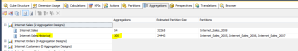
Updating the row and member counts used to be a very time consuming process. Thankfully, BIDSHelper introduced a feature, called Update Estimated Counts (screenshot below), that automates this process:

That said, there is currently no way to automatically update the partition count value (shown below) … which apparently can only be manually set via the Aggregation Design Wizard.

But based on the description of this field on MSDN and the comments in this thread by SQL Server MVP Deepak Puri (b | t), it seems this field only needs to be considered for the dimension (and relevant attributes) by which the target measure group is partitioned.

From the SSAS Performance Guide (referenced by Deepak in the thread linked above):

Whenever you use multiple partitions for a given measure group, ensure that you update the data statistics for each partition. More specifically, it is important to ensure that the partition data and member counts (such as EstimatedRows and EstimatedCount properties) accurately reflect the specific data in the partition and not the data across the entire measure group.

So while it’s a manual process, it shouldn’t be that bad since you’re only having to do it for a few attributes.

Considerations/Tips/Recommendations

Prior to starting this step, all dimensions should be properly reviewed. Any attributes that aren’t going to be used for slicing and dicing (ex. Customer Address, Customer Phone Number) should either be completely removed from the cube or the attribute hierarchies should be disabled (and accessed via member properties). This isn’t so much a tip directly related to Aggregation Design, but the implication is that it will reduce the number of attributes we need to evaluate.
When dealing with legitimate storage space and/or processing duration constraints from the get-go, be sure and deploy/process the cube prior to adding any initial aggregation designs to get an idea of the base data size. You might want to make some space saving adjustments to the base cube before wasting time adding aggregations that will likely push you over the space limit.
Use BIDSHelper to update the estimated counts of all your attributes before running the aggregation Aggregation Design Wizard. Generating the counts via the Aggregation Design Wizard has a few gotchas…mainly that the any existing non-zero counts won’t be updated. BIDSHelper, on the other hand, will update everything.
Consider creating separate Aggregation Designs for large partitioned measure groups where only a subset of partitions will be processed regularly. Older partitions that aren’t processed regularly can support heavier aggregation designs …assuming the space is available.
click to zoom
Don’t think too hard about which option to use on the Set Aggregation Options step of the Aggregation Design Wizard. Just follow the advice below from Expert Cube Development:

The approach we suggest taking here is to first select I Click Stop and then click the Start button. On some measure groups this will complete very quickly, with only a few small aggregations built. If that’s the case click Next; otherwise, if it’s taking too long or too many aggregations are being built, click Stop and then Reset, and then select Performance Gain Reaches and enter 30% and Start again. This should result in a reasonable selection of aggregations being built; in general around 50-100 aggregations is the maximum number you should be building for a measure group, and if 30% leaves you short of this try increasing the number by 10% until you feel comfortable with what you get.
Give the final aggregation design a descriptive name that references the measure group (and partition – where appropriate)… especially in scenarios where partition management is automated via SSIS/XMLA.
Save time during development by waiting until all initial aggregation designs have been created before deploying and processing…unless you are concerned about storage space and/or processing duration constraints, in which case you might considered deploying and processing after each measure group.

In the next post, we’ll focus on the second step in the ADLC where we detect and remove any unused aggregations…so state tuned!

One reply on “ADLC Step 1: Create Initial Aggregation Designs”

[…] 5) Use the Aggregation Design Wizard in SSAS to add multiple aggregations. This should be the first thing you do after a cube has been completed. See ADLC Step 1: Create Initial Aggregation Designs […]

LikeLike